Neural Networks Theory

Hello, hackers! Time for a small coffee break.

This is the first in a series of blog posts in which I’ll implement various deep learning algorithms and research papers. Before implementing anything new, I’ll explain the basic concept behind that. Knowledge of python and numpy are pre-requisites for this post.

The accompanying code can be found here. In the next post, I’ll do a line-by-line explanation of the code. This post covers the theory of a basic neural network.

The Brain and Artificial Neural Networks

Biological Neuron

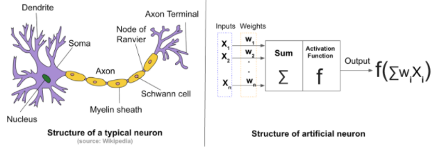
Brain consists of a number of brain cells (neurons) connected end-to-end. A neuron (Figure 2) takes electric impulse as signal, do some processing on the message, and send it to another neuron. So, a brain cell mainly consists of four parts:

1. Dendrites: Accepts inputs (electric impulses)

2. Soma: Process the inputs

3. Axon: Turn the processed inputs into a form that can be accepted by the next neuron i.e. converts processed inputs into output.

4. Synapses: The electrochemical contact between neurons. Using synapses, a neuron can transfer the outputs of that neuron to the inputs of the next neuron.

Artificial Neuron

To try to imitate the brain, “Artificial Neurons” were created with a similar structure.

Artificial neurons are extremely simplified versions of biological neurons. The inputs are represented by xi. Each input is “processed” i.e., multiplied by some weight wi, and all wixi products are added. After that, the processed input is passed through a function, known as the “activation function”, which converts the processed input to output. The value at the output of an artificial neuron is called the “activation” value. Finally, there is an output path.

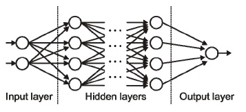
Figure 1: Architecture of ANN

These artificial neurons can be connected in many ways to give “artificial neural networks”. The example shown above is a shallow neural network. More layers of neurons can be added to make the network “deep”. Adding more layers (usually) increases the accuracy of the network. In such a network, there is one input layer, one or more hidden layers, and one output layer, as shown in Figure 1. The layers in between are called hidden layers because they are hidden from the user. Figure 2 shows the similarities between artificial and biological neurons.

Figure 2: Similarity between artificial and biological neurons

Working of Neural Networks

Components

Neural networks can (accurately) predict an output upon receiving some input. This section explores how it is done.

Broadly, a neural network consists of four components:

1. Artificial Neurons

2. Topology — how the neurons are connected

3. Weights

4. Learning algorithm

Forward Pass

Before the neural network can accurately predict the output, it needs to be trained on some data. Data usually consists of input-output pairs. The outputs in this dataset are known as “labels” or “targets”.

The “training” phase starts by randomly initialising all weights (i.e. weights associated with each artificial neuron). Then, inputs are fed to the network, activations of all nodes in hidden layers are calculated, and finally, we get the activation of the output layer (which is the actual output). The process described above is known as “forward pass”. Initially, the output is extremely inaccurate due to the random initialisation of the weights. The goal here is to finally arrive at an optimum value of the weights, such that the neural network can predict the output (given some input) with reasonable accuracy. The algorithm used to do this is known as “Backpropagation”.

Backpropagation

After the forward pass, we have some activations at the output layer. The output should ideally be equal to the label. However, that is not the case in the beginning, since the weights are randomly initisalized. So, error is calculated, and “backpropagated” through the network. The function that measures the error is known as the “cost function”. The aim is to adjust the weights to minimize this cost function. The technique used to minimize the cost function is called “gradient descent”.

Gradient Descent

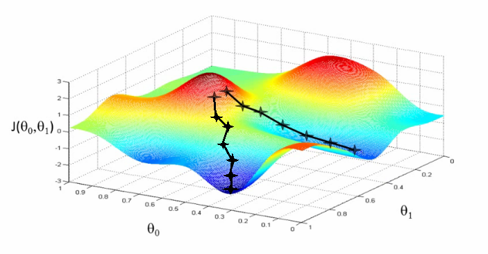
The plot of cost function vs weight is more or less convex and looks something like Figure 3:

Figure 3: Gradient Descent

The idea is that we make small steps in the direction of the gradient, and we hope that eventually, we’ll be at the global minima. However, that would be the case only if the plot is convex. Usually, the plot is not perfectly convex, resulting in a few local minima. For now, we’ll assume that the local minima are good approximations of the global minimum (which is usually the case).

So, we make small updates on the weights, each time moving them in the direction of the gradient. We multiply the updates with a parameter, known as “learning rate”.

This post gave a brief overview of the elements involved in making a neural network. Detailed analysis(and maths) of the algorithms will be done in separate posts.