Convolutional Neural Networks

Now that we understand backpropagation, let’s dive into Convolutional Neural Networks (CNNs)!

Code for visualization can be found here

Intuition

• Applying feedforward networks to images was extremely difficult. The number of parameters associated with such a network was huge. A better, improved network was needed specifically for images.

• Hubel and Wiesel performed experiments that gave some intuition about how images are biologically processed by the brain. They found that the brain responded in specific ways when it saw edges, patterns, etc. The visusal cortex was reported to be divided into layers, where the layers to the front recognized simple features like edges, but layers to the back recognized more complicated features.

Concepts

• Filters

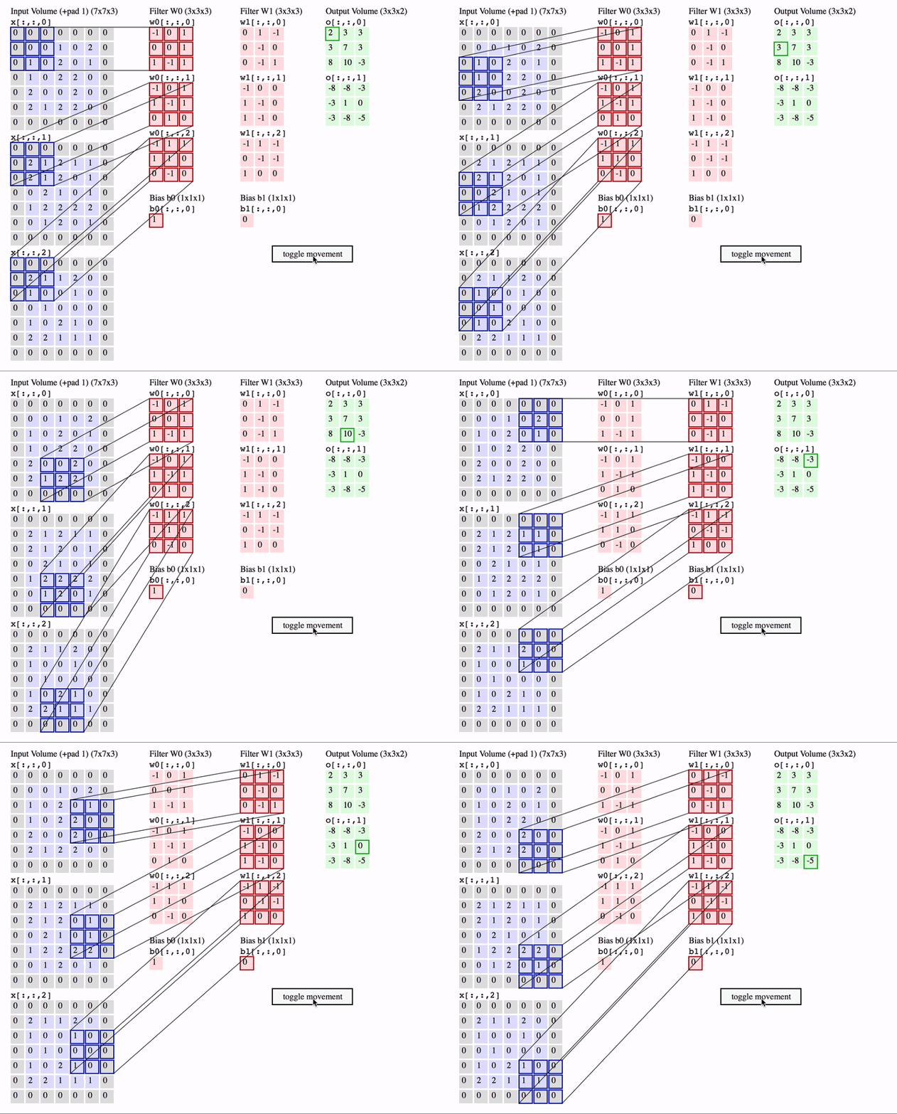
The basic concept behind CNNs is filters/kernels. You can think of them as smaller sized images which are then slided over the input image. By sliding over, I mean that the same filter is multiplied to different regions in the image (i.e. convolved over the image).

Images are represented by an array of shape (height, width, depth/channels), where there are 3 channels (RGB) for colour images, and 1 channel for grayscale images. For a filter to be able to “convolve” over the image, it should have the same number of channels as the input. The output is the sum of the elementwise multiplication of the filter elements and the image (can be thought of as dot product).

So, we can use any number of filters. The output depth dimension will be equal to the number of filters we use.

Source: http://cs231n.github.io/convolutional-networks/

In the above animation, two filters are being used. Notice that the depth (or channel) dimension of each filter is same as the depth of input (in this case, 3). The convolution operation is also clearly depicted in the animation. The output depth dimension is equal to the number of filters (in this case, 2). The output is the sum of the element-wise multiplication of filter and image over all channels (plus some optional bias term). So, it can be thought of as the dot product over the 3x3x3 (filter_height *filter_width * input_depth) volume.

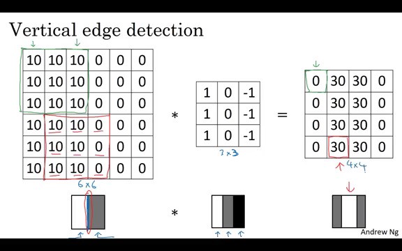
To get better intuition of filters, let’s look at an example of a filter that detects vertical edges.

Source: https://www.coursera.org/learn/convolutional-neural-networks/lecture/4Trod/edge-detection-example

The filter can be thought of as detecting some part of the image that is lighter to the left and darker to the right.

Sliding the filters also give an additional advantage of translation invariance, because the same features can be detected anywhere, irrespective of where they are present in the image.

Also, in practice, it is found that the initial layers tend to learn simpler features like edges, corners, etc. whereas the deeper layers tend to learn complex features like eyes, lips, face, etc.

Intuitively, it can be thought that we are combining the lower level features (eg. edges), and these combinations are resulting in a mixture of such features, thus resulting in higher level features. An oversimplified example would be, somehow combining two edge detecting filters to detect corners:

This is just for intuition (made using awwapp.com)

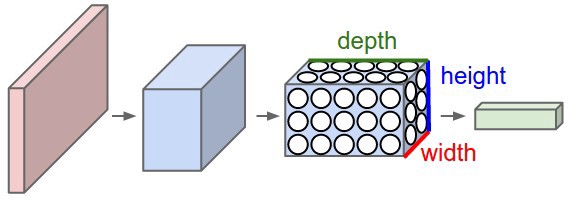
Hence, a complete convnet typically looks like this:

Source: http://cs231n.github.io/convolutional-networks/

Filters are randomly initialized, and are then learned via backpropagation.

• Layers

There are mainly 4 types of layers in CNNs:

1. Conv layers : These layers perform the convolution operation, as described above. The number of learnable parameters in these layers is equal to the number of parameters in each filter multiplied by the number of filters i.e. filter_height * filter_width * number_of_filters

2. Non-linearity : Conv layers are typically followed by a non-linearity layer. Usually ReLU is used. There are no learnable parameters in this layer.

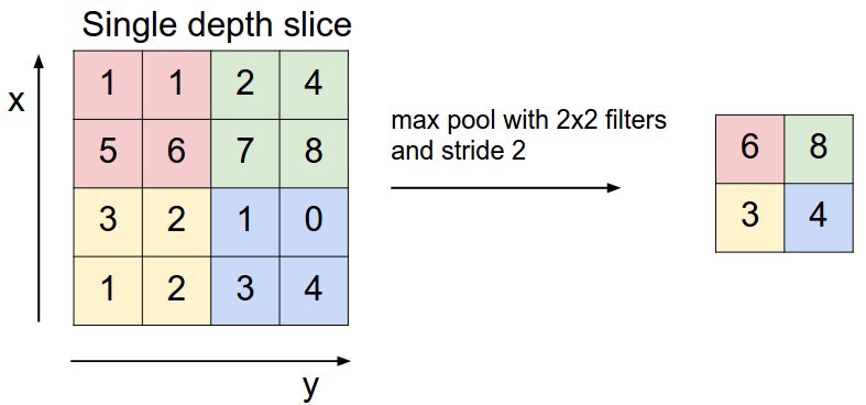
3. Pooling layer : This layer is used to downsample the image. It results in lesser parameters in the next layers, and hence the convnet can be made a little more deep.

Source: http://cs231n.github.io/convolutional-networks/

In theory, average pooling looks like the best option i.e. taking parts of the image, and averaging out that part to give one pixel value for that part of the image. But in practice, it was found that max-pooling works better, i.e. taking the maximum from that region in the image. Pooling layers maintain the depth dimension, i.e. pooling is done independently on all channels of the input. There are no learnable parameters in this layer.

1. Fully connected : These are usually at the end of the convnet. They are simple feedforward layers, and have as many learnable parameters as a normal feedforward net would have.

• Padding

One might argue that according to the convolution operation described above, the edges and corners of the image are getting lesser importance than the part in the middle of the image. To overcome this, the input is often zero-padded, i.e. a layer of zeros is added to all sides of the image. Also, zero-padding allows us to alter the size of the output image according to the requirement.

• Stride

The size of the jump while sliding the filter over the image is called stride. The more the stride, the smaller the output image will be.

The formula for calculating size of next layer after a conv layer is ((W−F+2P)/S)+1, where where W is the size of the image (width for horizontal dimension, and height for vertical dimension), F is the size of filter, P is the padding and S is the stride.

Another cool think to note is that as we move deeper into the network, the effective receptive field of the nodes increases, i.e. the node can be thought of as looking at a larger part of the image as compared to the layer before it.

Backpropagation

Backprop is done normally like a feedforward neural network. Derivatives of all weights (or parameters) are calculated w.r.t. loss, and are updated by gradient descent (or some variations of gradient descent, which will be discussed in a later post).

While applying the chain rule to find gradients w.r.t. loss, the gradient of one weight will come from all the nodes in the next layer to which the weight had contributed in the forward pass (It’ll be the sum of all these gradients, according to the multivariate chain rule of differentiation).

Visualization

Now that we understand how a convnet works, let’s try to visualize some of the stuff that happens inside the convnet.

An awesome explanation of some of the famous network architectures can be found here.

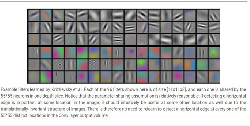
Visualizing weights of VGG neworks is not of much use, since the filters are only 3x3 in size. However, alexnet has 11x11 sized filters. The following image shows some filters learnt by alexnet.

Source: http://cs231n.github.io/convolutional-networks/

From this point on, all visualizations are done on VGG16 in Pytorch. The code can be found here.

So, let’s see what the output of each layer looks like:

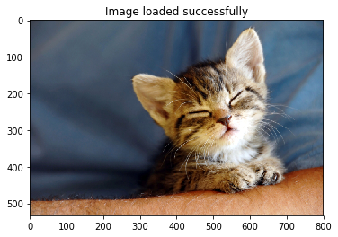
Input image:

Output at various layers:

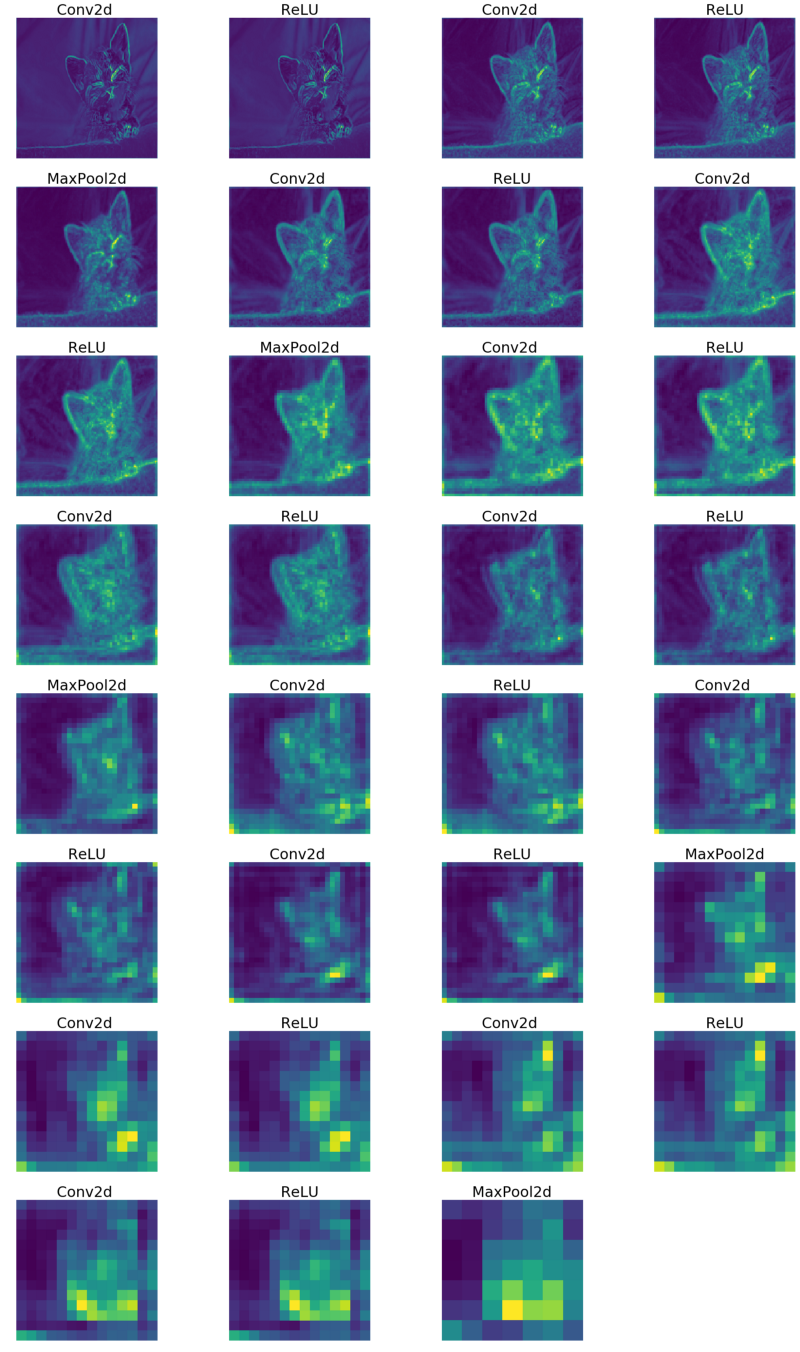
Since the number of channels at every layer are different (not 1 or 3), I’ve averaged over all channels to finally give a grayscale image (the color scheme is because of the default cmap scheme used by matplotlib).

Notice that maxpooling is simply downsampling the image.

If we don’t take average over all channels, we can see the output ofeach channel (i.e. output of each filter) at a particular layer. Let’s have a look:

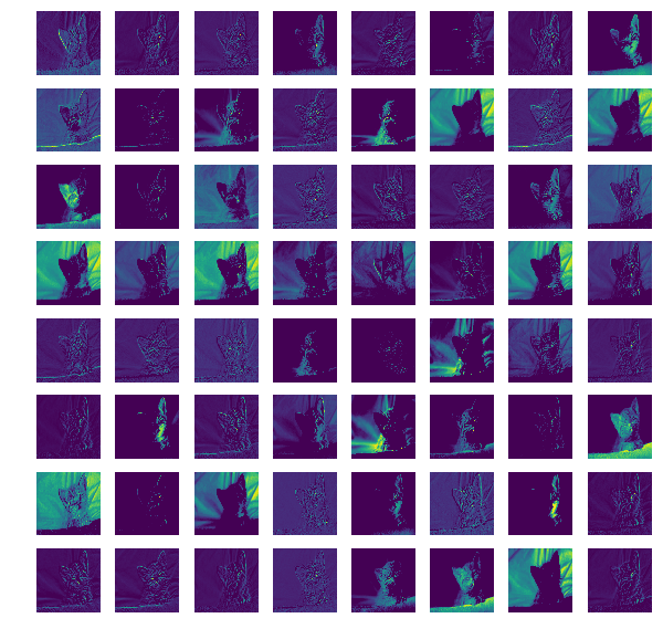
Output from first conv layer filters (all 64 channels from this layer)

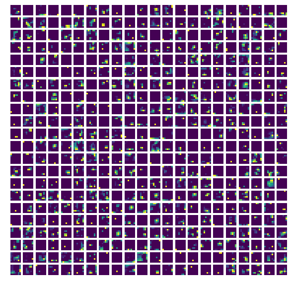
Output from last conv layer filters (first 484 channels are shown out of the total 512 channels at this layer)

We’ve seen the outputs from the filters, now let’s see what the filters actually look like:

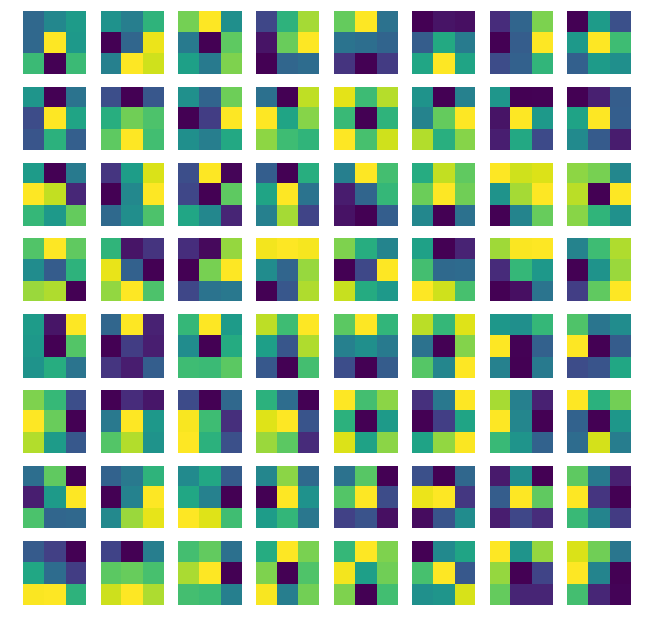
3x3 filters from first conv layer (64 filters)

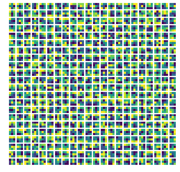
3x3 filters from last conv layer (first 484 out of total 512 filters at this layer)

Occlusion

Now let’s try to see actually what part of the image is responsible for the classification of an image.

First, I used a technique called occlusion. In this, we simply remove a region from an image, and then find the classification probability of the image being the true class. We do this for a lot of regions from the image (basically, we remove regions by slide over the entire image).

If the probability score comes out to be high, then we know that the blacked out region isn’t important for classification; the image is getting correctly classified without that region. If the probability comes out to be low, it means that the blacked out region was somehow important for correctly classifying the image.

The blue portion indicates low output score probability, and the yellow region shows high output class probability. So, the blue part depicts the parts that are important for classification.

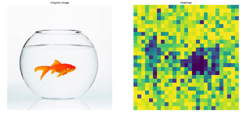
Occlusion Heatmap

Pretty impressive, right?

But the results are not so good, and the algorithm takes a lot of time to run (because it runs forward pass for classification too many times).

So, we try a different approach.

Saliency Maps

The concept behind saliency maps is simple. We find the derivatives of input image w.r.t. output score for an (image, class) pair. By definition, the derivative tells us the rate of change of classification score w.r.t. that pixel.

That is, how much the output class score will change if we change a particular pixel in the input image.

Here are some examples:

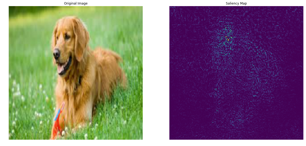
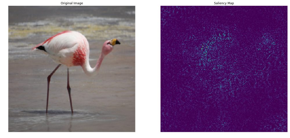
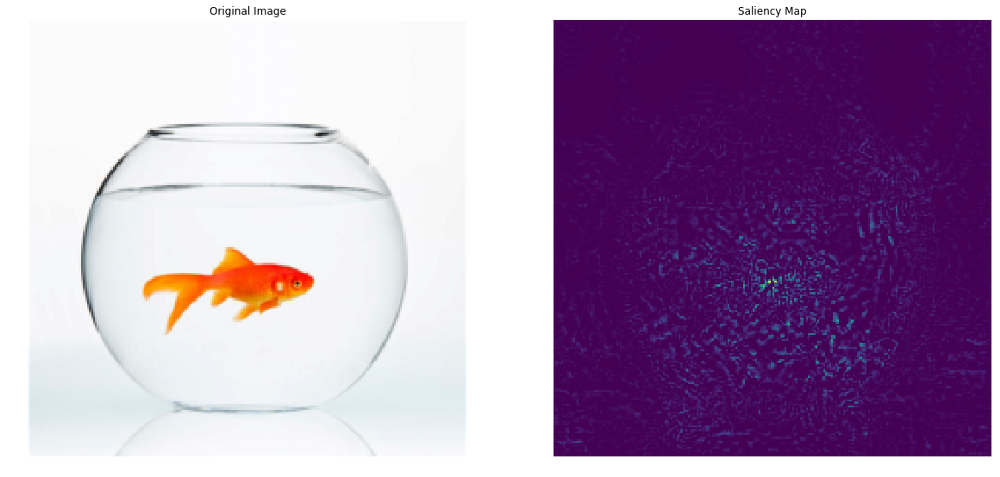
This runs extremely quick, and the results are pretty okay. But as you can see, there is a still huge room for improvement.

SmoothGrad

We can improve saliency maps (also called sensitivity maps) using SmoothGrad technique. I would like to quote the authors of this paper here:

“The apparent noise one sees in a sensitivity map may be due to essentially meaningless local variations in partial derivatives. After all, given typical training techniques there is no reason to expect derivatives to vary smoothly.”

The authors added some noise to the image and plotted the derivatives of the three channels (RGB) w.r.t. the output class score:

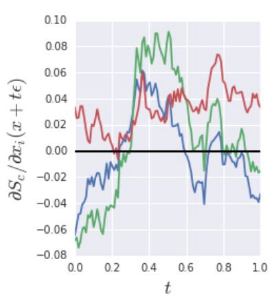
Source: https://arxiv.org/pdf/1706.03825.pdf (The original SmoothGrad paper)

Here, t determines the amount of noise to be added to the image. After adding a little bit of noise, the image appears not to change at all to the naked eye, i.e. it seems to be the same image, which is obvious. However, the derivatives of the input image fluctuate a lot.

So, the authors proposed that we do multiple iterations, and for every iteration, add a little bit of random noise to the original image. We’ll calculate the derivates of the input image (with added noise) for every iteration, and then finally take average of these derivatives before plotting it.

In the average, only those pixels will have high value of corresponding derivatives that had high value in every iteration. So, meaningless local variations in the derivatives will be removed.

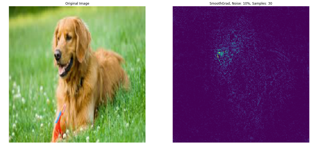
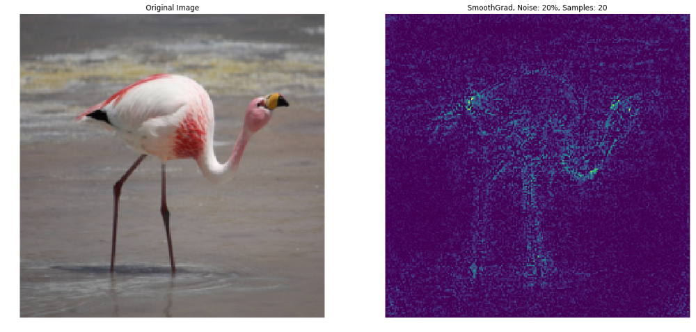
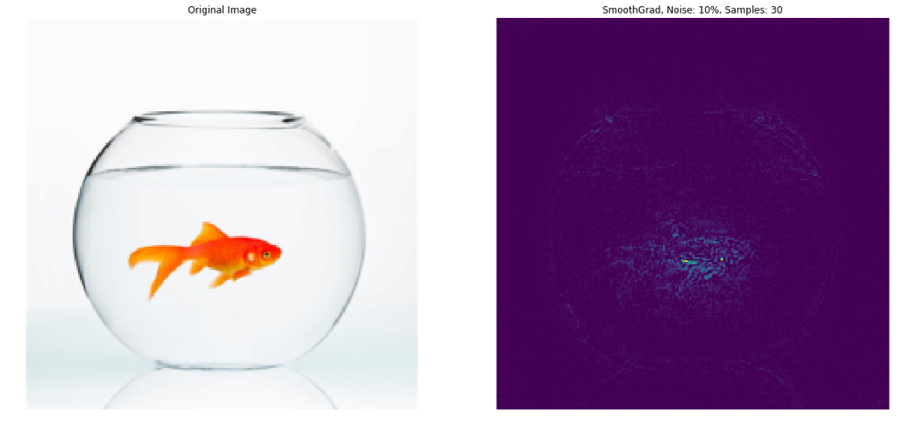
As you can see, the results are much better than simple saliency maps.

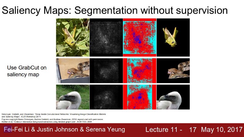
These techniques are extremely useful and can be used for semantic segmentation using GrabCut algorithm (which I haven’t implemented myself yet).

Image Source