Backpropagation

This would require a little bit of maths, so basic calculus is a pre-requisite.

In this post, I’ll try to explain backprop with a very simple neural network, shown below:

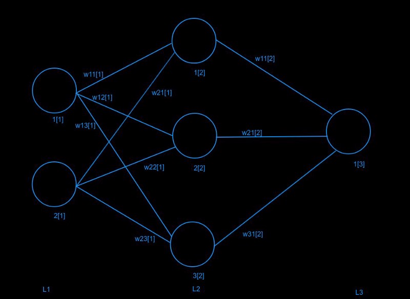
L1, L2 and L3 represent the layers in the neural net. The numbers in square bracket represent the layer number. I’ve numbered every node on each layer. E.g. second node of first layer is numbered as 2[1], and so on. I’ve labelled every weight too. E.g. the weight connecting second node of second layer (2[2]) to first node of third layer (1[3]) is w21[2].

I’ll assume that we’re using activation function g(z).

The basic concept behind backpropagation is to calculate error derivatives. After the forward pass through the net, we calculate the error, and then update the weights through gradient descent (using the error derivatives calculated by backprop).

If you understand chain rule in differentiation, you’ll easily understand backpropagation.

First, let us write the equations for the forward pass.

Let x1and x2 be the inputs at L1.

I’m denoting z as the weighted sum of previous layer, and a as the output of a node after applying non-linearity/activation function g.

z1[2] = w11[1]x1 + w21[1]x2

a1[2] = g(z1[2])

z2[2] = w12[1]x1 + w22[1]x2

a2[2] = g(z2[2])

z3[2] = w13[1]x1 + w23[1]x2

a3[2] = g(z3[2])

z1[3] = w11[2]a1[2] + w21[2]a2[2] + w31[2]*a3[2]

a1[3] = g(z1[3])

Now I’ll use MSE as a loss function.

E = (1/2)×(a1[3]−t1)², where t1 is the target label.

To use gradient descent to backpropagate through the net, we’ll have to calculate the derivative of this error w.r.t. every weight, and then perform weight updates.

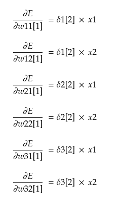
We need to find dE/dwij[k], where, wij is a weight at layer k.

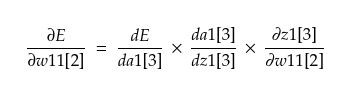
By chain rule, we have

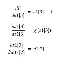
Now, we can calculate these three terms on the RHS as follows,

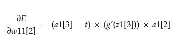
Therefore, we have

Similarly,

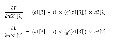
Let δ1[3] = (a1[3] — t) * (g’(z1[3])).

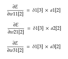
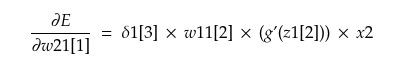
Hence, we have

Here, we’ll call δ1[3] as the error propagated by node 1 of layer 3.

Now, we want to go one layer back.

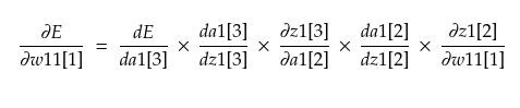
On simplifying, we get

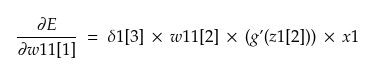
NOTE: The value of weight w11[2] is to be used before the update was performed on it. This applies to all equations and weights below.

Similarly,

Similarly backpropagating through other nodes in L2, we get

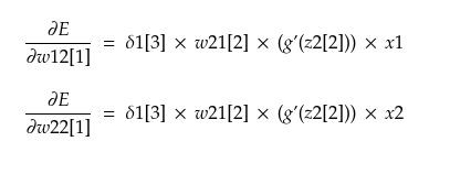
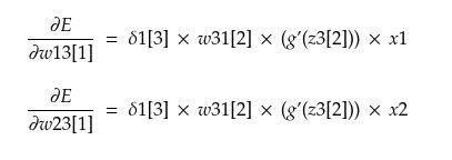
In terms of δ, these can be written as

When we have all the error derivatives, weights are updated as:

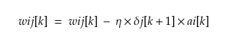
(wij[k] refers to weight wij at layer k)

where η is called the ‘learning rate’,

So, this was backprop for you!

To get a better grasp of this, you can try deriving it yourself.

You can even do it for some other error functions like cross-entropy loss (with softmax). Or for a particular activation function like sigmoid, tanh, relu or leaky rely.