Gradient Descent

Time for a break, coders! Let’s dive into a little bit of maths, shall we? insert nerdy smile

To understand gradient descent, let’s conisder linear regression. Linear regression is a technique, where given some data points, we try to fit a line through those points and then make predictions by extrapolating that line. The challenge is to find the best fit for the line. For the sake of simplicity, we’ll assume that the output(y) depends on just one input variable(x) i.e. the data points given to us are of the form (x, y).

Now we want to fit a line through these data points. The line will obviously be of the form y = mx + b, and we want to find the best values for m and b. This line is called our “hypothesis”.

To get started with, m and b are randomly initialized. Hence, we get a random line in the beginning. Our goal is to update these values so that the resulting line gives least error. We’ll use mean squared error as the cost function(J), that calculates the error between the actual value output, and prediction from the hypothesis.

J(m, b) = (1/n) * ∑(yᵢ - (mxᵢ + b))²

where n represents the total number of data points and i represents the iᵗʰ data point (i takes values from 1 to n).

This error function is typically convex. In simple terms, we can say that this error function typically has just one minimum (the global minimum).

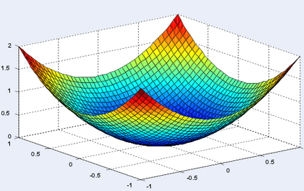
Figure: A convex function

The horizontal axes represent the variables on which the function depends, and the vertical dimension represents the output. In our case, the horizontal axes are represented by m and b, while the vertical axis is represented by y.

When we start with random values of m and b, we get some value of y correspondingly. Error is minimum at the lowest point on this graph, so our goal is to move down the slope to finally reach the bottom-most point. The question is, how?

Before moving on, I’d like you to recall some of your high school maths.

The slope of the tangent at any point on a graph is equal to the derivative of the graph w.r.t. input variables.

Image source

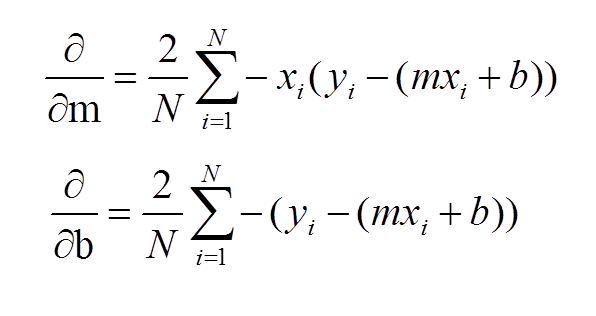
Now, as you can see, the slope of tangent at the bottom-most point on the graph is 0 i.e. partial derivatives of J at the bottom-most point are 0. To get to the bottom-most point, we have to move in the direction of the slope i.e. we’ll update values of m and b, such that we eventually get to the optimum values, where error function is minimum.

The update equations would be as follows:

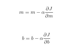
Here, α is called the “learning rate”, and it decides how large steps to take in the direction of the gradient. If the value of α is very small, reaching the optimum value is guaranteed, but it’ll take a lot of time to converge. If α is very large, then the values of m and b might overshoot the optimal values, and then the error will start to increase instead of decreasing. Hence, learning rate plays an important part in convex optimization.

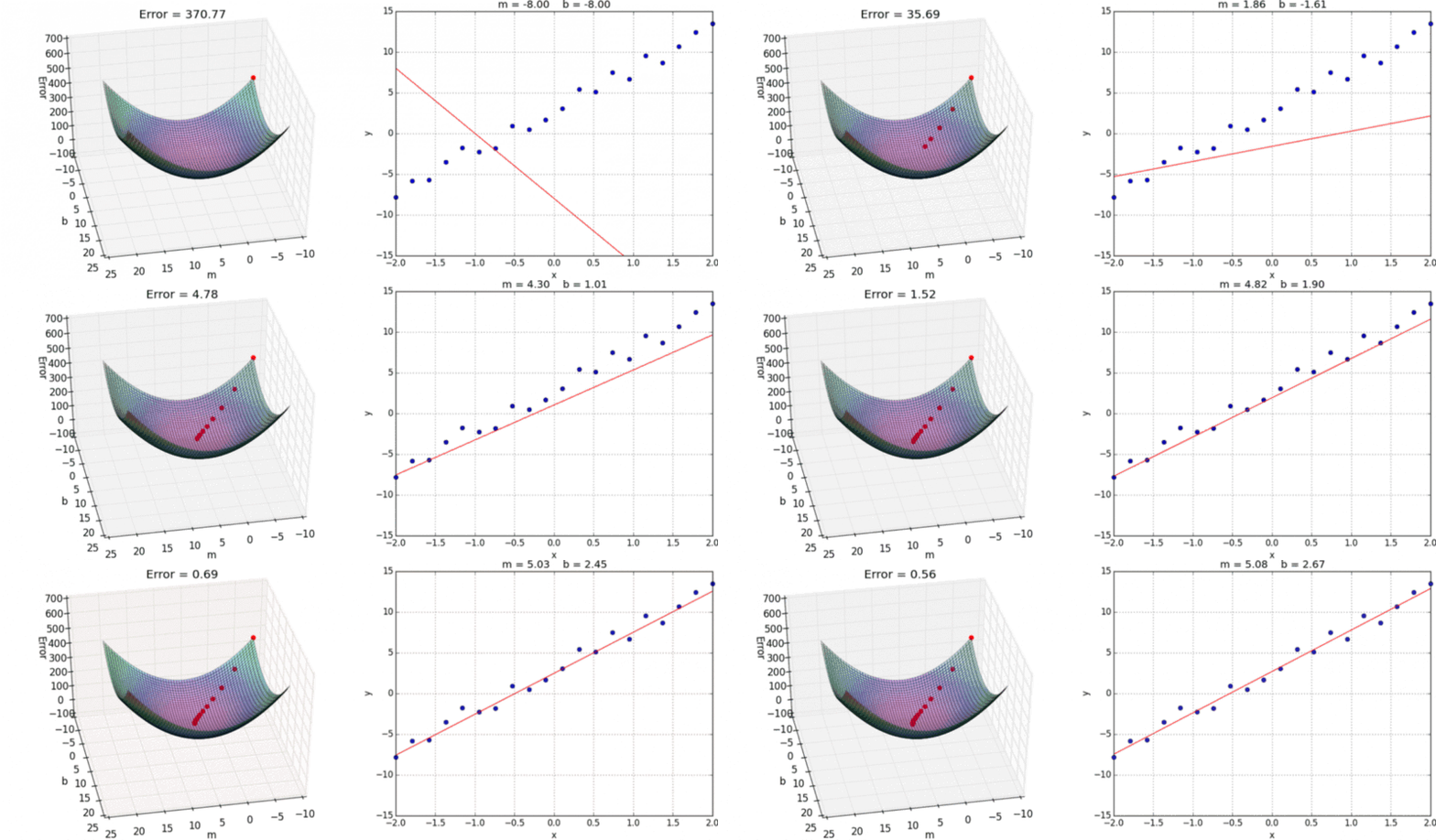
A visual representation of gradient descent in action has been shown below:

Image Source

How does it work intuitively?

For the sake of simplicity, consider an error function J that depends on only one variable (or weight) w.

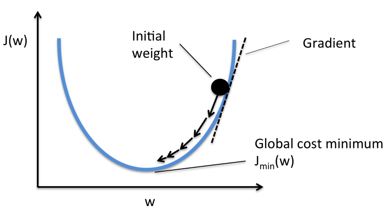
Consider the situation as shown in figure i.e. initial weight is more than the optimal value. Here, initially the slope is large and positive. So, in the update equation, w is reduced. As w keeps getting reduced, notice that the gradient also reduces, and hence the updates become smaller and smaller and eventually, it converges to the minimum.

Now consider the situation when the initial weight is less than the optimal value. Here, the slope is negative. So, in the update equation, the value of w increases after every update. Initially, the slope is large, so the updates are large. As w gets increased, the slope keeps getting smaller, and hence the updates keep getting smaller and eventually converge to the minimum.

So, in any case, the weights will finally converge to a value such that the derivative of the cost function is 0 (given that the value of alpha is sufficiently less).

In this post, I covered gradient descent for linear regression. However, this is the basic idea behind neural networks too. All the weights in the neural network are updated according to this algorithm. Gradient descent is used for optimization in the backpropagation algorithm.

Gradient Descent 101: Sometimes the smallest step in the right direction ends up being the biggest step of your life.